Morse Functions and Changes in Topology
1. Motivation and Justifications for the Study of Zeros of Functions
A smooth function filters a manifold by its sublevel sets. As the level rises through an interval without critical values, gradient flow can identify the levels under suitable compactness hypotheses. At a nondegenerate critical point, the Hessian describes the local change. Morse theory uses these local changes to study the topology of the manifold.
To motivate the study of connections between geometry and topology, let \(X\) be a complete differentiable manifold. Let \(f\) be a smooth real-valued function on \(X\). The essential feature of this theory and its generalizations is the relationship between the structure of the critical set of \(f\),
the space of trajectories for the gradient flow of \(f\), and the topology of \(X\). Informally, we can see the features of this theory in an example as follows. Let us consider a compact Riemannian manifold \(X\), which is diffeomorphic to \(\mathbb S^2\), and we study smooth functions on \(X\). As a foundation to this theory, we want to extract information about the global topology of \(X\) from the critical points of \(f\). Clearly, this number is not a topological invariant. One way in which we can distinguish topological features is, to each critical point \(p\), assign the number of linearly independent directions on which the second derivative \(\dif^{\:2}\! f(p)\) is negative definite. The study of Morse theory, therefore, immediately contains a series of local questions. We begin with the local behaviour of the gradient flow and then describe how crossing a critical value attaches a handle.
Definition 1. A \(C^2\) function \(f\) on a finite-dimensional smooth manifold \(X\) is Morse if its Hessian is nondegenerate at every critical point. At a critical point \(p\), the Hessian defines the linear isomorphism \(A:T_pX\to T_p^*X\), \(A(u)(v)=d^2f_p(u,v)\). Neither completeness nor a Riemannian metric is needed for this definition. Below, functions are smooth when smooth normal forms and flows are used.
Definition 2. The Morse index \(\mu(p)\) is the largest dimension of a linear subspace on which \(d^2f_p\) is negative definite. After choosing an inner product, it is the number of negative eigenvalues of the associated self-adjoint operator, counted with multiplicity. Sylvester's law of inertia makes this number independent of that choice and of coordinates. Thus \(0\le\mu(p)\le\dim X\), including index zero, and \(\operatorname{Crit}_k(f)\) denotes the critical points of index \(k\).
After choosing a Riemannian metric, the negative gradient flow solves
It is defined on an open maximal domain \(\mathcal D\subset\mathbb R\times X\), not necessarily on all of \(\mathbb R\times X\). Local ODE existence and uniqueness give the flow law whenever both sides are defined. The time-\(t\) map is a diffeomorphism between its open domain and the domain of the inverse time-\((-t)\) map. Along a trajectory,
Compactness of \(X\) guarantees existence for all time. Completeness of the Riemannian metric alone does not: on complete \(\mathbb R\), the function \(f(x)=-x^3/3\) has negative gradient \(x^2\), whose solution from \(x>0\) escapes in finite positive time.
With this in mind, we can then study the main features of Morse theory through a simple example: let \(X\) be a compact Riemannian manifold that is diffeomorphic to \(\mathbb S^2 \subset \mathbb R^3\). The goal is to study all smooth functions defined on \(X\). We seek information about the global topology of \(X\) from the critical points of smooth functions \(f\). It is clear that the number of critical points is not an invariant: this is why we wanted to define the Morse index to begin with (Definition 2). The motivation is clear through the following functions \(f_1\) and \(f_2\), illustrated in the figure below.
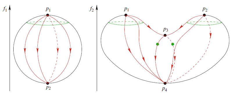
For the value \(p_1\), the Morse index of \(p_1\) associated with the function \(f_1\) is \(\mu_{f_1} (p_1) = 2\), because there are two linearly independent directions for which the negative gradient flow (flowing “downwards”) goes away from the critical point (\(p_1\) is the global maximum). Likewise, \(\mu_{f_2} (p_1) = \mu_{f_2} (p_2) = 2\), while \(\mu_{f_1} (p_2) = \mu_{f_2} (p_4) = 0\) and \(\mu_{f_2} (p_3) = 1\). In light of this example, let us look at the following objects.
Definition 3. The stable and unstable manifolds at \(x_0 \in X\) of the flow \(\varphi\) are defined as
Here \(x_0\) is a critical point, and the definition includes existence of the trajectory for all forward times in the stable case and all backward times in the unstable case. Initially these are sets; their manifold structure is a theorem, not a consequence of their definition.
For this topological conclusion, assume that \(X\) is compact without boundary and \(f\) is a smooth Morse function. Its critical points are isolated and form a closed set, hence there are finitely many. The Morse cell-attachment theorem gives a finite CW complex homotopy equivalent to \(X\), with one cell of dimension \(\mu(p)\) for each critical point \(p\). Write \(c_k(f)=\#\operatorname{Crit}_k(f)\). Each \(k\)-cell contributes \((-1)^k\) to the Euler characteristic, so the contribution of a critical point is determined by the parity of its index:
The equality is the alternating sum of the numbers of critical points of each index. For example, a height function on \(\mathbb S^2\) has one minimum and one maximum, contributing \(1+1=2\). The cell-attachment theorem is the topological input here; see Cohen, Iga and Norbury, Topics in Morse Theory, Introduction, Theorem 1.
The finite CW model gives a precise chain complex over \(\mathbb Z_2\). Its group \(C_k\) has one generator for each index-\(k\) critical point; the cellular attaching maps define \(\partial_k:C_k\to C_{k-1}\), with \(\partial_{k-1}\partial_k=0\). Consequently
The differential is not determined just by the list of critical points. Describing it by counting gradient trajectories requires a Morse–Smale transversality hypothesis and a separate compactness argument; the cellular definition suffices here.
The local stable-manifold argument explains the role of the Hessian. In coordinates centered at a nondegenerate critical point, with the metric Euclidean at that point, write the negative gradient vector field as
On a small convex ball the mean value estimate gives \(|\eta(x)-\eta(y)|\le\delta(\varepsilon)|x-y|\), where \(\delta(\varepsilon)\to0\) as \(\varepsilon\to0\). This is a local coordinate remainder, not a map \(X\to X\). Split into the stable and unstable eigenspaces \(E_s,E_u\), with \(A_s\le-aI\), \(A_u\ge aI\), \(a>0\). After a cutoff with sufficiently small Lipschitz norm, a bounded forward solution with stable initial coordinate \(s\) must satisfy
The second formula follows from variation of constants and boundedness as \(t\to\infty\). The right side is a contraction on bounded continuous paths when \(2\operatorname{Lip}(\eta)/a<1\). It is also a contraction in the weighted norm \(\sup_{t\ge0}e^{\beta t}|z(t)|\), for \(0<\beta<a\) and sufficiently small remainder, because the integral bound is \(\operatorname{Lip}(\eta)((a-\beta)^{-1}+(a+\beta)^{-1})\). Its unique fixed point therefore decays exponentially. Smooth parameter dependence of this contraction gives a smooth graph \(z_u(0)=h(s)\); differentiating at \(s=0\) gives \(Dh(0)=0\). This proves that the local stable set is a disk tangent to \(E_s\), of dimension \(\dim X-\mu(p)\). Reversing time gives the unstable disk of dimension \(\mu(p)\). The global stable and unstable sets acquire their immersed manifold structures by pulling back these disks along the flow. Local sets require trajectories to stay in the coordinate neighborhood; they are not identical to the global sets.
For a metric chosen Euclidean in Morse coordinates, the same conclusion is explicit: \(z_-(t)=e^{2t}z_-(0)\) and \(z_+(t)=e^{-2t}z_+(0)\). The local stable disk is \(z_-=0\), and the local unstable disk is \(z_+=0\). This supplies the geometric interpretation of the indices in the figure.
2. Morse Functions
We next check which features of critical points are independent of coordinates for a function \(f\) on a manifold. The following local results concern critical points of a function \(f\) on a manifold \(M\).
Lemma 4. Let \(f: M \to \mathbb R\) be a smooth function on a differentiable manifold \(M\). The critical points of \(f\) are independent of the chart chosen for \(M\).
Proof. On the overlap of charts, put \(F=f\circ\varphi^{-1}\), \(G=f\circ\psi^{-1}\), and \(h=\varphi\circ\psi^{-1}\). These functions are defined on the chart images, and \(G=F\circ h\). The chain rule gives \(dG_y=dF_{h(y)}\circ dh_y\). Since the smooth transition map has invertible derivative, one differential vanishes if and only if the other does. At a critical point, the second derivative chain rule reduces to
since the term involving \(dF\) vanishes. Hence the critical Hessian is a coordinate-independent bilinear form, and its nondegeneracy and index are intrinsic. \(\square\)
Lemma 5. Every nondegenerate critical point of a smooth function \(f:M\to\mathbb R\) is isolated. In particular, all critical points of a Morse function are isolated.
Proof. Choose coordinates centred at a nondegenerate critical point \(p\), and write \(F=f\circ\varphi^{-1}\). Consider the coordinate derivative map \(G=(\partial_1F,\ldots,\partial_nF)\). Then \(G(0)=0\), and \(DG(0)\) is the invertible Hessian matrix of \(F\) at \(0\). The inverse function theorem makes \(G\) injective on a neighbourhood of \(0\). Hence \(G(x)=0\) only at \(x=0\) in that neighbourhood, proving isolation. A nondegenerate critical point need not be a local extremum: \(F(x,y)=x^2-y^2\) has a nondegenerate saddle at the origin. ◻
A more general fact about vanishing derivatives is the following.
Lemma 6. Let \(f\) be smooth and let \(\ell\ge0\) be an integer. If all partial derivatives of orders \(1,\ldots,\ell\) vanish at \(p\) in one chart, they vanish at \(p\) in every chart. For \(\ell=0\), the assertion is vacuous.
In a chart \(\varphi\) centered at \(p\), the hypothesis is
Proof. Write \(G=F\circ h\) for the coordinate transition. Repeated use of the product and chain rules shows inductively that every derivative of \(G\) of order \(r\ge1\) is a sum of terms, each containing a derivative \(D^sF\) with \(1\le s\le r\), evaluated at \(h(y)\), multiplied by derivatives of \(h\). For \(r\le\ell\), each such factor vanishes at \(p\). This proves the claim from the hypothesis in one chart; it does not assume it in both charts. \(\square\)
Theorem 7 (Morse–Sard–Federer). Let \(f:M^m\to N^n\) be smooth, \(n\ge1\), and let
be its set of critical values. Then \(\dim_H\Delta_f\le n-1\), in particular \(\Delta_f\) has zero \(n\)-dimensional measure in smooth charts. Regular values are dense in \(N\), and regular values belonging to \(f(M)\) are dense in \(\operatorname{int}f(M)\).
This is a theorem used here. To explain the dimension conclusion, if \(m\ge n\), the finite-regularity bound gives \(\dim_H\Delta_f\le n-1+(m-n+1)/k\) for every \(k\); smoothness lets \(k\to\infty\). If \(m<n\), local Lipschitzness gives \(\dim_H f(M)\le m\le n-1\). Countably many relatively compact charts pass these bounds to manifolds. See Hajłasz, Korobkov and Kristensen, Theorem B, p.2. A measure-zero subset cannot contain an open set, giving the density assertion. It does not imply density of regular values inside every lower-dimensional portion of the image.
On a compact manifold, Morse functions form an open dense subset of smooth functions in the \(C^2\) topology. On a noncompact manifold, openness requires an appropriate strong topology and does not follow in the compact-open topology. The parameter argument below proves that sufficiently large smooth families have Morse members for almost every parameter. To see this, for a smooth, connected \(n\)-dimensional manifold \(M\), we will:
describe families of smooth functions \(f: M \to \mathbb R\) such that they depend smoothly on \(\lambda \in \Lambda\) (where \(\Lambda\) is a smooth, finite-dimensional manifold);
determine smooth map \(\pi : Z \to \Lambda\) such that \(f_\lambda\) is a Morse function for every regular value of \(\pi\);
apply Sard’s theorem to conclude that \(f_\lambda\) is “almost-everywhere” a Morse function.
Embed \(M^m\) in a finite-dimensional Euclidean space \(E=\mathbb R^N\); Whitney's embedding theorem supplies such an embedding. For a smooth family \(F:\Lambda\times E\to\mathbb R\), set \(F_\lambda(x)=F(\lambda,x)\) and \(f_\lambda=F_\lambda|_M\). Restriction of covectors is the surjective linear map \(P_x:E^*\to T_x^*M\), and
The family may also be specified intrinsically on \(\Lambda\times M\); the proof below only uses this partial differential.
Definition 8. The family of parametrized functions \(F: \Lambda \times E \to \mathbb R\) is sufficiently large relative to the submanifold \(M \hookrightarrow E\) if \(\dim \Lambda \geq \dim M\), and for all \(x \in M\), \(0 \in T_x^* M\) is a regular value for \(\partial^x f\). Furthermore, \(F\) is large if for every \(x \in E\) the partial differential map \(\partial^x F : \Lambda \to E^* : \lambda \mapsto \dif F_\lambda (x)\) is a submersion (in other words, if the differential at any \(\lambda \in \Lambda\) is surjective).
Lemma 9. If \(F : \Lambda \times E \to \mathbb R\) is large, then it is sufficiently large relative to any submanifold \(M \hookrightarrow E\).
Proof. By definition, since \(\partial^x F\) is a submersion, it follows that \(\partial^x f = P_x \dif F_\lambda (x)\) is a composition of two surjective differential maps (i.e. submersions), which is therefore a submersion. Therefore, \(\partial^x f\) has no critical values, therefore \(0\) has to be a regular value for \(\partial^x f\). ◻
Example 10 (Large families). The family \(H(\lambda,x)=\lambda(x)\), \(\lambda\in E^*\), has \(\partial^xH(\lambda)=\lambda\). Its parameter derivative is the identity, so it is large.
Let \(\Lambda\) be the open cone of positive definite symmetric operators on \(E\), and \(F(D,x)=\frac12\langle Dx,x\rangle\). At fixed \(x\ne0\), the derivative of \(D\mapsto Dx\) is \(A\mapsto Ax\), for arbitrary symmetric tangent operators \(A\). This derivative is surjective: for any \(y\in E\), the symmetric operator
satisfies \(Ax=y\), where \((u\otimes v)w=u\langle v,w\rangle\). Thus the family is sufficiently large on any submanifold avoiding \(0\). The map \(D\mapsto Dx\) itself is not onto \(E\), since \(\langle Dx,x\rangle>0\); it is its derivative that is onto. At \(x=0\), that derivative is zero, so the family is not large on all of \(E\).
The exceptional set in the next theorem is a set of parameters. Every resulting \(f_\lambda\) is defined on all of \(M\).
Theorem 11. If the family \(F:\Lambda \times E \to \mathbb R\) is sufficiently large relative to the submanifold \(M \hookrightarrow E\), then there exists a negligible set \(\Lambda_0\) such that for all \(\lambda \in \Lambda \setminus \Lambda_0\), the function \(f_\lambda : M \to \mathbb R\) is a Morse function.
Proof. In local coordinates on \(M^m\), form \(G(\lambda,x)=(\partial_{x^1}f_\lambda,\ldots,\partial_{x^m}f_\lambda)\). At \(G=0\), the parameter derivative \(D_\lambda G\) is onto by sufficient largeness. Thus the critical-pair set \(Z=\{(\lambda,x):df_\lambda(x)=0\}\) is a smooth submanifold of dimension \(\dim\Lambda\), by the regular value theorem. This description is independent of the trivialization of \(T^*M\).
Consider the projection \(\pi:Z\to\Lambda\). A tangent pair \((a,v)\) belongs to \(T_{(\lambda,x)}Z\) exactly when
Therefore \(d\pi\) is onto if the Hessian is invertible. Conversely, if \(d\pi\) is onto, every \(a\) can occur in such a tangent pair. Since \(D_\lambda G\) is onto, the Hessian must be onto, hence invertible. Thus \(\lambda\) is a regular value of \(\pi\) exactly when all critical points of \(f_\lambda\) are nondegenerate. Sard's theorem makes the set of nonregular values negligible in parameter charts, proving the claim. Empty critical fibers cause no problem.
For completeness, compact-manifold density follows by applying this to \(f_\lambda=f+\lambda\circ i\), where \(i:M\hookrightarrow E\) is an embedding: parameter derivatives span every cotangent space, and arbitrarily small good \(\lambda\) give arbitrarily small \(C^2\) perturbations on compact \(M\). Openness follows by taking small neighborhoods of the finitely many critical points where the Hessians remain nonsingular, and using a positive lower bound for \(|df|\) on their compact complement. Sufficiently small \(C^2\) perturbations preserve both properties. \(\square\)
3. Morse Functions and Their Topology
There are two steps in describing sublevel sets. First consider intervals without critical values; then examine the change across one critical value:
“Weak” Morse principle: if \(f^{-1}([a,b])\) is compact and contains no critical points, the sublevels \(M^t=\{f\leq t\}\), \(a\leq t\leq b\), are diffeomorphic by a suitably normalized gradient flow. Compactness prevents finite-time escape while traversing this strip.
“Strong” Morse principle: crossing a nondegenerate critical point of index \(\lambda\), isolated in a compact strip, attaches a \(\lambda\)-handle to the sublevel. Its boundary undergoes the corresponding surgery. These are assertions about \(\{f\leq t\}\), with the handle dimension determined by the number of negative Hessian directions.
We introduce the topological constructions needed to state the change across a critical value precisely.
A closed \(k\)-cell is a copy of \(\mathbb D^k\), and attaching it to a space \(A\) along \(\phi:\mathbb S^{k-1}\to A\) forms the quotient \(A\cup_\phi\mathbb D^k\). Finite CW complexes are built inductively in this way, attaching boundaries to lower-dimensional skeleta.
Surgery on a smooth \(m\)-manifold uses an embedded \(k\)-sphere, \(0\le k<m\), together with a framing of its rank-\((m-k)\) normal bundle. A tubular-neighborhood embedding \(\phi:\mathbb D^{m-k}\times\mathbb S^k\to M\) then specifies the replacement
Both boundaries are \(\mathbb S^{m-k-1}\times\mathbb S^k\), of dimension \(m-1\). Collars on the two sides identify a neighborhood of the seam with this boundary times an open interval, giving the glued smooth structure. Thus it is the disk of dimension \(k+1\), not \(k-1\), that fills each copy of the surgery sphere. Isotopic framed embeddings give diffeomorphic surgeries, by extending the isotopy to the tubular neighborhood.
For a manifold with boundary, a \(\lambda\)-handle of dimension \(m\) is \(\mathbb D^\lambda\times\mathbb D^{m-\lambda}\), attached along \(\partial\mathbb D^\lambda\times\mathbb D^{m-\lambda}\) in the boundary. Corners can be rounded; the induced boundary change is surgery.
A smooth Morse function is exhaustive if every sublevel \(M^c=\{f\le c\}\) is compact. A vector field \(X\) is gradient-like in the increasing direction if \(df(X)>0\) away from critical points and in Morse coordinates \(f=f(p)-|x_-|^2+|x_+|^2\) it equals
Here \(0\le\lambda\le m\); either sum may be empty.
Remark 12. Morse coordinates exist by the Morse lemma: a smooth function with a nondegenerate critical point of index \(\lambda\) has local form \(f(p)-|x_-|^2+|x_+|^2\). The linear-algebra step is coordinate invariant by Lemma 4. One construction writes \(f-f(p)=\sum a_{ij}(x)x^ix^j\) using Taylor's integral remainder; the symmetric matrix \(a(0)\) is half the nonsingular Hessian. Successively completing squares with nonzero pivots, shrinking the neighborhood at each step, gives smooth coordinate changes with invertible derivative. Sylvester's law gives exactly \(\lambda\) negative squares. This is the Morse lemma used in the handle argument.
Choose a metric equal to the Euclidean metric in smaller Morse-coordinate neighborhoods. Such a metric exists: the critical set is closed and discrete, so choose disjoint locally finite coordinate neighborhoods, use cutoffs equal to one on smaller neighborhoods, and patch their Euclidean metrics to any initial metric by convex combinations. Positive definite forms remain positive definite under these combinations. In general coordinates,
For the adapted metric this becomes the gradient-like field displayed above. Its negative flow in the coordinate neighborhood is
This formula is valid while the trajectory remains in the coordinate neighborhood. It verifies directly the stable and unstable dimensions and the sign convention.
With these descriptions, and the regular-interval lemma (Lemma 10 of the isotopy-lemma note), we can state and prove the fundamental structural theorem.
Theorem 13 (Fundamental structural theorem). Suppose \(c\) is a critical value of \(f\) containing a single critical point \(p\) of Morse index \(\lambda\). Then, for every \(\varepsilon > 0\) sufficiently small, the sublevel set \(\{f \leq c+\varepsilon\}\) is homeomorphic to \(\{f \leq c-\varepsilon\}\) with a \(\lambda\)-handle of dimension \(m\) attached. If \(x = (x_-,x_+)\) are coordinates adapted to the critical point, then the core of the handle is given by \(e_\lambda (p) \triangleq \{x_+ = 0 ~,~ |x_-|^2 \leq \varepsilon\}\). In particular, \(\{f \leq c+\varepsilon\}\) is homotopic to \(\{f \leq c-\varepsilon\}\) with the \(\lambda\)-cell \(e_\lambda\) attached.
Assume here that \(f\) is smooth and exhaustive on a manifold without boundary. Equivalently for this local crossing argument, it suffices that a slightly larger strip around \(c\) be compact and contain no other critical points. The two endpoint levels are regular. “Homotopic to” means “homotopy equivalent to,” and the handle attachment is understood with corners rounded.
Proof. Choose a Morse-coordinate neighborhood \(U\) of \(p\). Compactness of a strip and isolation of critical points let us choose \(\varepsilon>0\) so that \(p\) is the only critical point in the strip and the closed coordinate ball \(B\triangleq\{|x_-|^2+|x_+|^2\le2\varepsilon\}\) lies in \(U\).
To apply the weak Morse principle across the critical level \(c\) without altering the topology of the upper sublevel set, we construct an auxiliary smooth function \(F : M \to \mathbb{R}\). We want \(F\) to match \(f\) outside \(B\), but strictly lower the critical value at \(p\) to push it below \(c-\varepsilon\). Let \(\mu : [0, \infty) \to [0, \infty)\) be a smooth bump function satisfying the following criteria:
\(\mu(0) > \varepsilon\),
\(\mu(r) = 0\) for all \(r \geq 2\varepsilon\),
\(-1 < \mu'(r) \leq 0\) for all \(r \geq 0\).
Such a bump exists: take a smooth \(h:[0,2\varepsilon]\to[0,1)\), vanishing near \(2\varepsilon\), whose integral exceeds \(\varepsilon\), and let \(\mu(r)=\int_r^{2\varepsilon}h(s)\,ds\) for \(r<2\varepsilon\), extended by zero. Then \(\mu'=-h\) has the required bounds. Define \(F=f-\mu(|x_-|^2+2|x_+|^2)\) in \(U\), and \(F=f\) elsewhere.
Because \(\mu(r) = 0\) for \(r \geq 2\varepsilon\), \(F\) is a well-defined smooth function that transitions identically to \(f\) on and outside the boundary of \(B\). Furthermore, since \(\mu \geq 0\), we have \(F(x) \leq f(x)\) everywhere.
We first claim that \(\{f \leq c+\varepsilon\} = \{F \leq c+\varepsilon\}\). The condition \(F \leq f\) trivially implies \(\{f \leq c+\varepsilon\} \subseteq \{F \leq c+\varepsilon\}\). For the reverse inclusion, assume for the sake of contradiction there exists an \(x \in M\) such that \(F(x) \leq c+\varepsilon\) but \(f(x) > c+\varepsilon\). This discrepancy requires \(x \in B\) and the argument of \(\mu\) to be strictly less than \(2\varepsilon\), meaning \(|x_-|^2 + 2|x_+|^2 < 2\varepsilon\). This enforces that \(2|x_+|^2 \leq |x_-|^2 + 2|x_+|^2 < 2\varepsilon\), and consequently \(|x_+|^2 < \varepsilon\). However, substituting this into the local form of \(f\) yields:
which contradicts \(f(x) > c+\varepsilon\). Thus, the sublevel sets are strictly identical: \(\{f \leq c+\varepsilon\} = \{F \leq c+\varepsilon\}\).
Next, we verify that \(F\) has no critical values in the closed interval \([c-\varepsilon, c+\varepsilon]\). Outside \(B\), \(F = f\), which has no critical points in this bounded range. Inside \(B\), we compute the partial derivatives of \(F\):
Because \(-1<\mu'\le0\), both \(1+\mu'\) and \(1-2\mu'\) are positive, so the only critical point of \(F\) in the coordinate ball is \(p\), with \(F(p)=c-\mu(0)<c-\varepsilon\). Outside the ball, \(F=f\). Consequently the compact strip \(F^{-1}([c-\varepsilon,c+\varepsilon])\) has no critical points. The regular-interval lemma gives both a diffeomorphism of its endpoint sublevels and a strong deformation retraction of the upper sublevel onto the lower one. Since the upper \(F\)- and \(f\)-sublevels agree, it remains to identify the lower \(F\)-sublevel.
We now prove the cell conclusion without assuming a handle retracts onto its core while fixing its entire attaching region. Put \(A=\{f\le c-\varepsilon\}\), \(u=x_-\), \(v=x_+\), \(a=|u|^2\), and \(b=|v|^2\). On the new region \(\{F\le c-\varepsilon\}\setminus A\), hold \(u\) fixed and shrink \(v\) until its squared norm is
More explicitly, for \(b>0\) replace \(v\) by \(\bigl((1-t)+t\sqrt{b_*/b}\bigr)v\), \(0\le t\le1\). Fix \(A\) pointwise, and also fix \(v=0\). On the new region \(b>b_*\), so this shrinks \(b\); since \(\partial F/\partial b=1-2\mu'>0\), it stays in the sublevel. At the interface with \(A\), the factor is \(1\); at \(v=0\), continuity follows because the displacement is bounded by \(|v|\). The deformation is supported inside the coordinate ball and pastes continuously to the identity outside it.
At time one, if \(a>\varepsilon\) the point lies on \(f=c-\varepsilon\); if \(a\le\varepsilon\), it lies on the core disk \(e_\lambda=\{v=0,\ |u|^2\le\varepsilon\}\). The whole core lies in the \(F\)-sublevel because \(a+\mu(a)\ge\mu(0)>\varepsilon\), using \(1+\mu'>0\). This is a strong deformation retraction onto \(A\cup e_\lambda\), fixing both \(A\) and the core. Composing with the regular-strip retraction proves the claimed cell attachment and its attaching sphere \(|u|^2=\varepsilon,\ v=0\).
For the stronger handle description, choose \(0<\delta<\varepsilon\) small and use the actual product neighborhood
The map \((w,v)\mapsto(\sqrt{\varepsilon+|v|^2}\,w,v)\) identifies it with \(\mathbb D^\lambda\times\mathbb D_{\sqrt\delta}^{m-\lambda}\). Its intersection with \(A\) is precisely \(|w|=1\), so it is a handle attached along the required product of sphere and disk. Its core is \(e_\lambda\). Choose the chart large enough to contain this small handle.
Outside \(A\cup H_\delta\), the compact strip has no critical points. The negative adapted gradient decreases both \(f\) and \(|v|^2\) in the chart, with derivatives \(-4(|u|^2+|v|^2)\) and \(-4|v|^2\). It therefore crosses inward through each exposed face of \(A\cup H_\delta\), namely \(f=c-\varepsilon\) or \(|v|^2=\delta\). Rounding their common corner preserves this transversality. Every descending trajectory from the upper level reaches this boundary in finite time: otherwise it would remain in a compact region where \(|\nabla f|\) has a positive lower bound while \(f\) decreases indefinitely. Conversely, the reversed flow reaches the upper level. Smooth dependence and the implicit function theorem for the transverse hitting time identify the region between the rounded boundary and the upper level with a product collar. Rescaling this collar and using the identity farther inside gives a diffeomorphism from the upper sublevel to \(A\) with this handle attached, after rounding corners. For \(\lambda=0\) the handle is a new disk with empty attaching region; for \(\lambda=m\) its entire boundary attaches. These endpoint cases follow from the same local quadratic model. \(\square\)
Reading: Carmo (1992), Riemannian geometry.